The Dirac equation (1): introduction

Although it took me much more time than I expected, the introductory part of the notes on the Dirac equation is ready. I welcome all comments.

In order to properly understand the Dirac equation, one needs some background on the Lorentz transformation. In this post, we also discuss briefly some aspects of Maxwell’s equations, which will become important later when we couple the Dirac particle with electromagnetic field.

1. Notation

To keep the notes readable for mathematicians, it is important to keep the notation as simple and as consistent as possible. In quantum mechanics, the state of a particle (or a system of particles) at time $t$ is described completely by an element $\psi(t)$ of a fixed Hilbert space $\mathcal{H}$ with norm $1$ . (This definition is already not strictly Lorentz-invariant; we will discuss this later.) In the Dirac model, $\mathcal{H} = (L^2(\mathbf{R^3}))^4$ is the space of square-integrable $\mathbf{C}^4$ -valued functions on $\mathbf{R^3}$ . Measurable values in this theory correspond to self-adjoint, typically unbounded linear operators on $\mathcal{H}$ , called observables. If, for example, $\vec{x}$ and $\vec{p}$ are the position and the momentum vectors of a classical particle, then we denote the corresponding observables by $\vec{\boldsymbol{x}}$ and $\vec{\boldsymbol{p}}$ .

Three-dimensional vectors (space vectors) are denoted by $\vec{x} = (x_1, x_2, x_3)$ , $\vec{p} = (p_1, p_2, p_3)$ etc. By $x$ , $p$ we denote the lenght of vectors $\vec{x}$ , $\vec{p}$ . Relativistic four-vectors are written in roman font, for example $\vec{\mathrm{x}} = (t, \vec{x}) = (t, x_1, x_2, x_3)$ . For that reason, we sometimes write $t = x_0$ . Mathematically, a four-vector is just a four-dimensional vector. We use the name four-vector to emphasize that a natural class of transformations acting on four-vectors is the group of Lorentz transformations (see below), and not isometries. The set of four-vectors is called space-time.

The partial derivative operators are denoted by $\partial_j$ ( $j = 1, 2, 3$ ). Furthermore, $\nabla = (\partial_1, \partial_2, \partial_3)$ is the vector of spatial partial derivatives and $\Delta = \partial_1^2 + \partial_2^2 + \partial_3^2$ is the spatial Laplace operator. The gradient of a function, divergence of a vector field, and its curl are denoted by $\nabla \varphi$ , $\nabla \cdot \vec{A}$ and $\nabla \times \vec{A}$ . The time derivative is denoted by $\partial_t$ , or $\partial_0$ when four-vectors are discussed. Sometimes we also use a dot placed over a symbol, like in $\dot{\psi}$ .

The evolution of the state is described by the wave function $\psi(t, \vec{x})$ . We often drop the arguments from the notation when they are clear from the context. Furthermore, we often write $\psi(t)$ for $\psi(t, \cdot)$ , a function of the spatial variable. Perhaps it is worth noting that the wave function typically does not satisfy the usual wave equation, but a Schrödinger one. 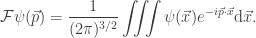As it was already mentioned, in the Dirac approach the function $\psi$ takes values in $\mathbf{C}^4$ , so that $\psi(t, \vec{x}) = (\psi_1(t, \vec{x}), \psi_2(t, \vec{x}), \psi_3(t, \vec{x}), \psi_4(t, \vec{x}))$ .

Physicists often use fixed variable names for fixed spaces, or representations. The symbol $\vec{x}$ corresponds to the position, and the wave function $\psi(t, \vec{x})$ is given in the so-called position (or standard) representation. However, it is often more convenient to work with the (spatial) Fourier transform of $\psi$ , which corresponds to the so-called momentum representation, related to the momentum variable $\vec{p}$ . Instead of writing the Fourier transform explicitly, it is customary to write simply $\psi(t, \vec{p})$ for the Fourier transform of $\psi$ . This is just a very convenient short hand notation, but at first it may seem very informal. For that reason, we try to avoid it, and write $\mathcal{F} \psi(t, \vec{p})$ instead. We use $\mathcal{F}$ for the Fourier transform normalized to be an $L^2$ isometry,

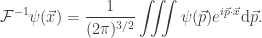
$\displaystyle \mathcal{F} \psi(\vec{p}) = \frac{1}{(2 \pi)^{3/2}} \iiint \psi(\vec{x}) e^{-i \vec{p} \cdot \vec{x}} \mathrm{d}\vec{x} .$

The inverse Fourier transform is then given by the formula

$\displaystyle \mathcal{F}^{-1} \psi(\vec{x}) = \frac{1}{(2 \pi)^{3/2}} \iiint \psi(\vec{p}) e^{i \vec{p} \cdot \vec{x}} \mathrm{d}\vec{p} .$

Finally, we choose to use natural units. That is, we choose unit system in such a way that some chosen physical constants are equal to one, thanks to which we can drop them from the formulas. We will assume that the speed of light $c$ , the electric and magnetic constants $\varepsilon_0$ and $\mu_0$ and the (reduced) Planck constant $\hbar$ are all equal to one.

2. Maxwell’s equations and Lorentz transformation

One of the main features of the Dirac equation is its Lorentz invariance: the Dirac equation has the same form in all inertial (in the sense of special relativity) frames of reference. It is therefore reasonable to start with a short introduction to the Lorentz transformation. And since its discovery was mostly motivated by Maxwell’s equations, we shall begin with a brief introduction to classical electromagnetism.

The evolution of the electric field $\vec{E}(t, \vec{x})$ and the magnetic field $\vec{B}(t, \vec{x})$ is described by the system of four Maxwell’s equations:

$\begin{cases} \nabla \cdot \vec{E} = \varrho, \\ \nabla \cdot \vec{B} = 0, \\ \nabla \times \vec{E} = -\partial_t \vec{B}, \\ \nabla \times \vec{B} = \partial_t \vec{E} + \vec{J}, \end{cases} \hspace{\stretch{1}} (2.1)$

where $\varrho(t, \vec{x})$ is the density of electric charge and $\vec{J}(t, \vec{x})$ is the density of electric current. These two objects are ruled by a rather complicated mechanism which depends on what type of media is the space filled with: conducting or not, magnetic or not etc. Here we will consider $\varrho$ and $\vec{J}$ simply to be parameters, describing an external source of electromagnetic wave, and only note the general continuity equation:

$\partial_t \varrho + \nabla \cdot \vec{J} = 0 . \hspace{\stretch{1}} (2.2)$

Intuitively, (2.2) is a form of electric charge conservation law: it says that $\vec{J}$ describes the flow of the electric charge $\varrho$ .

When there is no electric charge and no current, all components of $\vec{E}$ and $\vec{B}$ satisfy the classical wave equation: $\partial_t^2 \vec{E} = \Delta \vec{E}$ and $\partial_t^2 \vec{B} = \Delta \vec{B}$ . For example, using the identity $\nabla \times (\nabla \times \vec{E}) = \nabla (\nabla \cdot \vec{E}) - \Delta E$ , we obtain

$\partial_t^2 \vec{E} = -\partial_t (\nabla \times \vec{B}) = -\nabla \times \partial_t \vec{B} = -\nabla \times (\nabla \times \vec{E}) = \Delta \vec{E} - \nabla (\nabla \cdot \vec{E}) = \Delta \vec{E}.$

Maxwell’s equations agree perfectly with experimental data. However, they are not preserved by Galilean transformations. This is true even with the absence of electric charge and current, because Galilean transformations do not preserve the classical wave operator $\partial_t^2 - \Delta$ . It is not dificult to find linear transformation of coordinates preserving $\partial_t^2 - \Delta$ : the frame of reference moving with constant speed $v$ in the $x_1$ direction should be described by the Lorentz transformation (a Lorentz boost):

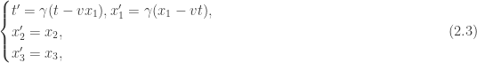
$\displaystyle \begin{cases} t' = \gamma(t - v x_1), x_1' = \gamma (x_1 - v t), \\ x_2' = x_2, \\ x_3' = x_3, \end{cases} \hspace{\stretch{1}} (2.3)$

where $\gamma = 1 / \sqrt{1 - v^2}$ is the Lorentz factor. It is an easy (but very instructive) exercise to verify explicitly that the transformation (2.3) indeed preserves the classical wave operator. The Lorentz boost corresponding to the frame of reference moving with arbitrary constant speed $\vec{v}$ can be obtained from (2.3) by rotations, but the result is not very simple:

$\displaystyle \begin{cases} t' = \gamma(t - \vec{v} \cdot \vec{x}), \\ \vec{x}' = \vec{x} + (\gamma - 1) \, \frac{\vec{v} \otimes \vec{v}}{v^2} \, \vec{x} - \gamma \vec{v} t, \end{cases} \hspace{\stretch{1}} (2.4)$

again with $\gamma = 1 / \sqrt{1 - v^2}$ . Here $\vec{v} \otimes \vec{v}$ is a $3 \times 3$ matrix with entries $v_i v_j$ , and $\vec{v} \otimes \vec{v} / v^2$ is the ortogonal projection on the line containing $\vec{v}$ . Lorentz boosts, rotations, translations and their compositions, form the group of Lorenz transformations of space-time. Since Lorenz transformation do not preserve time, they were first considered as a purely mathematical notion, and it was Albert Einstein who first considered them (in special relativity) to be the true physical description of inertial frames of reference.

There are two types of Lorentz invariance. Suppose that two inertial frames are related by a Lorentz boost (2.3). A path $\vec{\mathrm{x}}(s) = (x_0(s), x_1(s), x_2(s), x_3(s))$ (here $x_0$ corresponds to the time variable $t$ ) in the primed frame is given by $\vec{\mathrm{x}}'(s)$ , with

$x_0' = \gamma(x_0 - v x_1), \quad x_1' = \gamma (x_1 - v x_0), \quad x_2' = x_2, \quad x_3' = x_3 , \hspace{\stretch{1}} (2.5)$

and similar formula can be written for the derivatives of $\vec{\mathrm{x}}$ . Physicists say that four-vectors, such as $\vec{\mathrm{x}}$ and $\partial_s \vec{\mathrm{x}}$ , transform in a contravariant way. On the other hand, a function $f(x_0, x_1, x_2, x_3)$ (again $x_0$ is the time coordinate) in the primed frame is given by the formula $f'(x_0', x_1', x_2', x_3') = f(x_0, x_1, x_2, x_3)$ , so that its derivatives are transformed in a covariant way:

$\partial_0' f' = \gamma(\partial_0 + v \partial_1) f, \; \partial_1' f' = \gamma(\partial_1 + v \partial_0) f, \; \partial_2' f' = \partial_2 f, \; \partial_3' f' = \partial_3 f. \hspace{\stretch{1}} (2.6)$

This is a natural transformation for gradient-like operations. (The above discussion may seem completely trivial for most physicist. However, I always found this covariant and contravariant terminology quite confusing, so I hope such a lay explanation will help many mathematicians. At least, I needed it.)

It is perhaps surprising — it was for me — to note that Maxwell’s equations (2.2) (or, more precisely, the electric and magnetic fields) are not strictly invariant under the Lorentz transformation. The easiest way to see this is to consider a single stationary charge. Since it is at rest, it generates no current, and so the magnetic field is constant zero. On the other hand, in a different inertial frame, the charge is no longer stationary, the electric current is no longer zero, and so $\vec{B}$ cannot vanish. Therefore, the magnetic field cannot be measured absolutely, without fixing an inertial frame of reference. There are, however, relatively simple (but different from (2.5) and (2.6)) transformation rules for $\vec{E}$ and $\vec{B}$ , which is no longer true when Galilean transformation are considered.

What is Lorentz-invariant (well, contravariant) is the potential. To introduce this notion, we need the Helmholtz theorem. Informally, it states that any vector field can be written in the form $\nabla V + \nabla \times \vec{A}$ for some function $V$ (the scalar potential) and some vector field $\vec A$ (the vector potential). The first summand in the decomposition has no curl (it is irrotational), the other one has zero divergence (it is solenoidal).

The main topic of these notes is the Dirac equation, which deals with square integrable functions. Therefore, we give the simplest, $L^2$ version of Helmholtz Theorem instead of the ‘continuous’ version typical in electrodynamics. This way we also introduce the notion of Sobolev spaces, a very important object in quantum mechanics. A function $V$ is said to belong to the Sobolev space $H^k$ if $V$ and partial derivatives of $V$ of order up to $k$ (defined in the distributional sense) are square integrable. Equivalently, $V \in H^k$ if and only if $(1+p)^k \mathcal{F} V(\vec{p})$ is square integrable. A vector field is said to be square integrable etc., if so are all of its components.

Helmholtz Theorem
Suppose that $\vec{B}$ is a square integrable vector field. Suppose furthermore that $\iiint B_i \mathrm{d}\vec{x} = 0$ , and that $x B$ is integrable. Then there exist a function $V$ and a vector field $\vec{A}$ such that 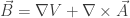$\vec{B} = \nabla V + \nabla \times \vec{A}$ . Furthermore, $V$ and each component of $\vec{A}$ are in the Sobolev space $H^1$ .

Sketch of the proof. By the assumptions, $\mathcal{F} \vec{B}(\vec{p})$ and $(1/p) \mathcal{F} \vec{B}(\vec{p})$ are square integrable. Define the potentials using the Fourier transform, by the formulas

$\mathcal{F} V(\vec{p}) = (-\mathrm{i} \vec{p} / p^2) \cdot \mathcal{F} \vec{B}(\vec{p}) , \qquad \mathcal{F} \vec{A}(\vec{p}) = (-\mathrm{i} \vec{p} / p^2) \times \mathcal{F} \vec{B}(\vec{p})$ ,

and verify the statements of the theorem. $\square$

In principle, the vector potential $\vec{A}$ is not defined uniquely: the curl is not changed when $\vec{A}$ is replaced by $\vec{A}' = \vec{A} + \nabla g$ for any function $g$ . Choosing a particular vector potential is known as gauge fixing. When $\vec{A}$ is the vector potential constructed in the proof of Helmholtz theorem, then $\nabla \cdot \vec{A} = 0$ . In this case we have $\Delta g = \nabla \cdot \vec{A}'$ . Hence, the function $g$ can be recovered from $\vec{A}'$ by the formula 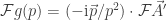$\mathcal{F} g(p) = (-\mathrm{i} \vec{p}/p^2) \cdot \mathcal{F} \vec{A}'$ . This means that gauge fixing is equivalent to an arbitrary choice of the divergence $\nabla \cdot \vec{A}$ of the vector potential.

We now come back to the electric and magnetic fields $\vec{E}, \vec{B}$ . Since $\nabla \cdot \vec{B} = 0$ , the magnetic field has zero scalar potential. Let $\vec{A}$ be a vector potential of $\vec{B}$ , the magnetic potential. The vector field $\partial_t \vec{A} - \vec{E}$ has zero curl, and therefore its vector potential vanishes. Let $V$ be the scalar potential of $\partial_t \vec{A} - \vec{E}$ , the electric potential. When fixing $\vec{A}$ , we use the Lorenz gauge (note that Ludvig Lorenz and Hendrik Lorentz were two different physicists): we require that

$\nabla \cdot \vec{A} + \partial_t V = 0 . \hspace{\stretch{1}} (2.7)$

Before we discuss why this condition can be satisfied, let us note that with the above definitions, we have

$\begin{cases} \vec{E} = - \nabla V - \partial_t \vec{A} , \\ \vec{B} = \nabla \times \vec{A} , \end{cases} \hspace{\stretch{1}} (2.8)$

and Maxwell’s equations (after some manipulation) can be rewritten as

$\begin{cases} \partial_t^2 \vec{A} - \Delta \vec{A} = \vec{J} , \\ \partial_t^2 V - \Delta V = \varrho , \end{cases} \hspace{\stretch{1}} (2.9)$

accompanied by the Lorenz gauge condition (2.7) and the continuity equation (2.2).

It was noted above that the classical wave operator is preserved by Lorentz transformations. This proves that the Maxwell’s equations (2.9) are Lorentz-invariant. On the other hand, (2.8) and (2.2) are not strictly Lorentz-invariant. In fact, these formulas say that $(V, \vec{A})$ and $(\varrho, \vec{J})$ are vector fields on space-time and transform according to (2.5). For $(\varrho, \vec{J})$ this is rather intuitive, and by (2.9), $(V, \vec{A})$ should transform in the same way. For this reason, it is sometimes convenient to define the electromagnetic four-potential $\vec{\mathrm{A}} = (A_0, A_1, A_2, A_3)$ by taking $A_0 = V$ . Then (2.9) reduces to a single equation

$\partial_t^2 \vec{\mathrm{A}} - \Delta \vec{\mathrm{A}} = \vec{\mathrm{J}} ,\hspace{\stretch{1}} (2.9')$

where $\vec{\mathrm{J}}$ is the four-current, with $J_0 = \varrho$ . Furthermore, the relation (2.8) can be written in a more abstract form using the electromagnetic tensor (the word matrix may sound more familiar here, though):

$\mathrm{F} = \begin{pmatrix} 0 & E_1 & E_2 & E_3 \\ -E_1 & 0 & -B_3 & B_2 \\ -E_2 & B_3 & 0 & -B_1 \\ -E_3 & -B_2 & B_1 & 0 \end{pmatrix} ,$

Formula (2.8) says that $F_{i,j} = \epsilon_i \partial_i A_j - \epsilon_j \partial_j A_i$ , where $\epsilon_0 = -1$ and $\epsilon_1 = \epsilon_2 = \epsilon_3 = 1$ . Also (2.1) could be written in terms of $\mathrm{F}$ , but it is no longer that elegant (see, for example, the Wikipedia article).

It remains to explain why the Lorentz gauge condition is in fact a gauge condition. The general magnetic and electric potentials, without fixing any gauge, can be described as follows. We start with the magnetic potential $\vec{A}_0$ with divergence zero and the corresponding electric potential $V_0$ . (This corresponds to the Coulomb gauge.) In general, we have $\vec{A} = \vec{A}_0 + \nabla g$ , where $g(t, \vec{x})$ is an arbitrary, sufficiently smooth function. It follows that $V = V_0 - \partial_t g$ . The Lorenz gauge condition can be rewritten as $\Delta g - \partial_t^2 g + \partial_t V_0 = 0$ , which transforms to an ordinary differential equation in the Fourier space, $p^2 \mathcal{F} g(\vec{p}) + \partial_t^2 (\mathcal{F} g)(\vec{p}) + \partial_t \mathcal{F} V_0(\vec{p}) = 0$ . General theory gives existence of a solution. Note that, however, $g$ is not defined uniquely: all Lorenz gauge functions differ from each other by a solution of the classical wave equation $\partial_t^2 \varphi = \Delta \varphi$ . Therefore, the pair $(V, \vec{A})$ of electric and magnetic potentials is defined uniquely up to the four-gradient of a solution of the classical wave equation: changing $V$ and $\vec{A}$ to $V - \partial_t \varphi$ and $\vec{A} + \nabla \varphi$ does not affect (2.7)–(2.9).

One thing should be pointed out here: we do not discuss any regularity properties (smoothness, square integrability etc.) of the solutions of Maxwell’s equations. This issue will be partially addressed later, when we will couple a wave function with electromagnetic field. However, we will usually assume that the potentials are smooth enough and consider them as parameters of the environment.

[table of contents|next]

	Alexander Perlis on Heronian triangles conjecture
	Mateusz Kwaśnicki on Mathematica and hypergeometric…
	juanmarqz on Mathematica and hypergeometric…
	mateuszkwasnicki on Heronian triangles conjecture
	Johannes boot on Heronian triangles conjecture